🎯 Support Vector Machine (SVM)
Machine Learning Made Simple
3-Minute Complete Guide
🤔 What is a Support Vector Machine?
A powerful classifier that finds the optimal boundary to separate classes with maximum margin.
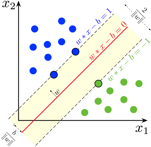
SVM finds the line with maximum margin between classes
Think of SVM like a referee in a sports game: It draws the fairest possible line between two teams, keeping maximum distance from both sides to avoid disputes. This "fairest line" is what makes SVM so powerful - it doesn't just separate classes, it does so with maximum confidence.

SVM vs other classifiers - notice the optimal margin
Why is this important? Imagine you're trying to separate emails into spam and not-spam. Other algorithms might draw any line that separates them, but SVM finds the line that's furthest away from both types of emails. This means when a new, uncertain email arrives, SVM is most likely to classify it correctly.
💻 How SVM Works

Step-by-step: How SVM finds the optimal decision boundary
The SVM Process Explained:
1. Identify Support Vectors: SVM looks at your data and finds the points that are closest to the boundary between different classes. These are called "support vectors" - think of them as the most important data points that will determine where the boundary goes.
2. Maximize the Margin: Instead of just drawing any line that separates the classes, SVM draws the line that is as far as possible from the support vectors on both sides. This creates the widest possible "safety zone" between classes.

Support vectors (circled points) determine the decision boundary
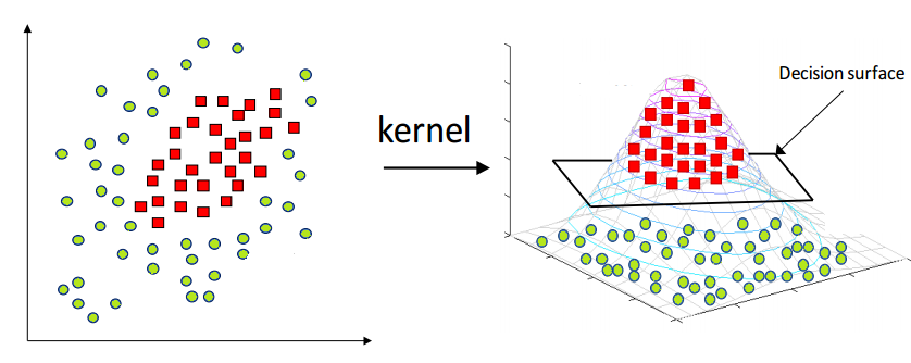
3. Handle Complex Data: When data isn't linearly separable (can't be separated by a straight line), SVM uses "kernels" to transform the data into higher dimensions where it becomes separable. It's like lifting a tangled rope into 3D space to untangle it.
🎯 SVM Kernels: The Magic Behind Complex Patterns

Different kernels handle different data patterns - from simple lines to complex curves
Understanding Kernels Through Real Examples:
Linear Kernel: Imagine trying to separate cats from dogs based on weight and height. If heavier, taller animals are mostly dogs and lighter, shorter ones are cats, a straight line can separate them perfectly. This is when you use a linear kernel.
Linear kernel (top) vs RBF kernel (bottom) - see how RBF handles curved boundaries
RBF (Radial Basis Function) Kernel: Now imagine the data is more complex - maybe small dogs and large cats exist too. The boundary becomes curved, like drawing circles around clusters. RBF kernel excels at this by creating flexible, curved decision boundaries.
Polynomial Kernel: Think of data that follows a specific mathematical pattern, like a parabola. Polynomial kernels can capture these specific curved relationships, making them perfect for certain scientific or engineering applications.

How kernels transform data: from non-separable to separable
SVC(kernel='rbf') # For complex, curved patterns (most common)
SVC(kernel='poly') # For specific polynomial relationships
⚡ Key Concepts: The Building Blocks of SVM
The anatomy of SVM: Support vectors, hyperplane, and margin
Support Vectors - The VIP Data Points:
Imagine you're organizing a party and need to put a rope barrier between two groups of people. You don't need to consider everyone - just the people standing closest to where the rope will go. These "closest people" are your support vectors. In SVM, these are the data points that actually matter for drawing the decision boundary. Remove any other point, and the boundary stays the same. Remove a support vector, and everything changes!

Support vectors (highlighted) are the only points that matter for the decision boundary
Hyperplane - The Ultimate Decision Maker:
In 2D, it's a line. In 3D, it's a flat surface. In higher dimensions, it's called a hyperplane. This is SVM's decision boundary - everything on one side gets classified as Class A, everything on the other side as Class B. The beauty is that SVM finds the hyperplane that's furthest from all the support vectors, making it the most confident decision possible.
Margin - The Confidence Zone:
The margin is like a "buffer zone" around the decision boundary. A wider margin means SVM is more confident about its decisions. It's the distance from the hyperplane to the nearest support vectors on each side. SVM's goal is to maximize this margin, creating the most robust classifier possible.
Wider margin = more confident predictions
🚀 Real-World Applications: Where SVM Shines

SVM successfully classifying the famous Iris dataset
Email Spam Detection:
Every day, your email provider uses algorithms like SVM to protect you from spam. SVM analyzes thousands of features in each email - word frequency, sender patterns, link density, and more. It creates a high-dimensional boundary that separates legitimate emails from spam with remarkable accuracy. The beauty is that SVM can handle the complexity of natural language without getting confused by new spam tactics.

SVM processing text data for classification
Medical Diagnosis:
Doctors use SVM-powered systems to analyze medical images, predict disease risks, and assist in diagnosis. For example, SVM can analyze thousands of features in a mammogram to detect early signs of breast cancer, often spotting patterns that human eyes might miss. The algorithm's ability to work with high-dimensional data makes it perfect for processing complex medical information.
Financial Fraud Detection:
Banks use SVM to detect fraudulent transactions in real-time. By analyzing spending patterns, location data, transaction amounts, and timing, SVM can instantly flag suspicious activities. Its ability to create complex decision boundaries helps it distinguish between legitimate unusual purchases and actual fraud attempts.
SVM creating optimal decision boundaries for complex real-world data
🎨 SVM Kernels in Action
🔧 Choosing the Right Kernel:
from sklearn.datasets import make_circles
# Create non-linearly separable data (circles)
X_circles, y_circles = make_circles(n_samples=100, noise=0.1, factor=0.3)
# Test different kernels
kernels = ['linear', 'rbf', 'poly']
for kernel in kernels:
svm = SVC(kernel=kernel, C=1.0)
svm.fit(X_circles, y_circles)
score = svm.score(X_circles, y_circles)
print(f"{kernel.upper()} kernel accuracy: {score:.3f}")
📊 Kernel Selection Guidelines:
🎯 When to Use Each Kernel:
- Linear: Large datasets, text classification
- RBF: Small-medium datasets, unknown patterns
- Polynomial: Image processing, specific domains
- Custom: Domain-specific problems
⚡ Performance Tips:
- Start with RBF: Good default choice
- Try Linear: If RBF is too slow
- Scale Features: Always normalize your data
- Tune Parameters: Use GridSearchCV
📈 SVM vs Other Algorithms: When to Choose What

Comparing SVM with other popular machine learning algorithms
SVM's Superpowers:
High-Dimensional Excellence: While other algorithms struggle when you have thousands of features (like in text analysis or genomics), SVM actually thrives. It's like having a superhero that gets stronger with more complexity. This makes SVM perfect for analyzing documents, DNA sequences, or any data with many features.
Memory Efficiency: Unlike algorithms that need to remember all your training data, SVM only remembers the support vectors - usually just a small fraction of your data. It's like having a brilliant student who only needs to remember the key points to ace any test.

SVM vs other classifiers on different types of datasets
SVM's Limitations:
Speed on Large Datasets: SVM is like a master craftsman - it produces excellent results but takes time with large projects. For datasets with millions of samples, faster algorithms like Random Forest might be better choices.
No Probability Scores: SVM tells you "this is spam" or "this is not spam" but doesn't tell you "I'm 85% confident this is spam." If you need probability estimates, algorithms like Logistic Regression might be more suitable.
Feature Scaling Sensitivity: SVM is like a precise instrument that needs calibration. You must scale your features (make them similar ranges) before using SVM, or it might focus too much on features with larger numbers.
The complete SVM workflow: from raw data to predictions
🛠️ Fine-Tuning SVM: The Art of Parameter Optimization

How C and gamma parameters dramatically affect SVM's decision boundary
The C Parameter - The Perfectionist vs The Flexible Friend:
Think of C as SVM's personality trait. A high C value makes SVM a perfectionist - it tries to classify every single training example correctly, even if it means creating a very complex boundary. This can lead to overfitting, like memorizing answers instead of understanding concepts.
A low C value makes SVM more flexible and forgiving. It's okay with making a few mistakes on training data if it means creating a simpler, more generalizable boundary. It's like a teacher who focuses on the big picture rather than nitpicking every detail.
Low C (left) vs High C (right) - notice how the boundary changes
The Gamma Parameter - Local vs Global Thinking:
Gamma controls how far the influence of a single training example reaches. High gamma means each point only influences its immediate neighborhood - like having very localized opinions. This creates complex, wiggly boundaries that can overfit.
Low gamma means each point has a far-reaching influence - like having a global perspective. This creates smoother, more generalized boundaries. It's the difference between a local neighborhood watch and a national security system.
Different gamma values create different decision boundaries
🎓 Next Steps & Best Practices
🚀 Advanced Techniques:
- Multi-class SVM: One-vs-One, One-vs-Rest
- SVM Regression: SVR for continuous predictions
- Online SVM: Incremental learning
- Ensemble Methods: Combine multiple SVMs
- Custom Kernels: Domain-specific functions
- Feature Selection: Reduce dimensionality
💡 Best Practices:
- Always Scale: Use StandardScaler or MinMaxScaler
- Cross-Validation: Use CV for parameter tuning
- Start Simple: Try linear kernel first
- Handle Imbalance: Use class_weight parameter
- Monitor Overfitting: Check validation scores
- Consider Alternatives: Random Forest for large data
💡 Practice Suggestions:
Try building SVM models for these problems:
- 🖼️ Image classification (handwritten digits)
- 📧 Spam email detection
- 🏥 Medical diagnosis systems
- 💰 Credit card fraud detection
- 📈 Stock market prediction
- 🎬 Movie sentiment analysis
⚠️ Important Reminders:
Always remember to:
- Scale your features before training SVM
- Use cross-validation for hyperparameter tuning
- Start with RBF kernel, then try linear for speed
- Monitor for overfitting with validation curves
- Consider computational cost for large datasets